
Lane change implementation through pure pursuit, stanley and Lateral Lane Changing Controller Design
Introduction
Path tracking refers to a vehicle tracks a globally specified geometric path by applying suitable steering movements that lead the vehicle along the path, and vehicle controllers are usually referred to as path trackers. The purpose of a path tracking controller is to reduce the lateral distance between the vehicle and the specified route, reduce the difference in the vehicle's heading and the defined path's heading, and keep the vehicle stable by limiting steering inputs to smooth movements. There are many different forms of vehicle controllers, but geometric path trackers are one of the most common types of path tracking technologies used in robotics. Geometric controllers construct control rules based on geometric correlations between the vehicle and the route. A look ahead distance is frequently used in these procedures to quantify inaccuracy ahead of the vehicle. Various courses are created to evaluate the controllers' characteristics and give insight into their respective benefits and drawbacks. This study will compare and evaluate two types of geometric controllers for a comparable route course, namely the Lane Change Course, which is a straight portion of two-lane road (Figure 1). The lane change manoeuvre, which is an important collision avoidance technique, is a standard vehicle handling test.
Problem/ Objective
Implement Pure Pursuit and Stanley Geometric Controllers for the Lane Change Course in MATLAB and simulate their behaviour in order to have a better knowledge of the steering and control models for wheeled mobile robots (WMR). A single lane change manoeuvre is required to demonstrate the vehicle's tracking capacity on a straight road as well as its response to a rapid, yet (position and curvature) continuous, transient segment. Path tracking is done using constant speeds of 5 m/s, 10 m/s, 15 m/s, and 20 m/s respectively.

Figure 1: Lane Change Course
Geometric Bicycle Model
The bicycle model is a typical approximation of an Ackerman steered vehicle used for geometric route tracking. By merging the two front wheels and the two rear wheels to make a two-wheeled vehicle, the bicycle model simplifies the four-wheeled car. The vehicle can only move on a plane, according to the second simplification. As a result of these simplifications, the front wheel steering angle and the curve that the rear axle will follow have a straightforward geometric connection. This basic geometric connection may be stated as seen in Figure 2.
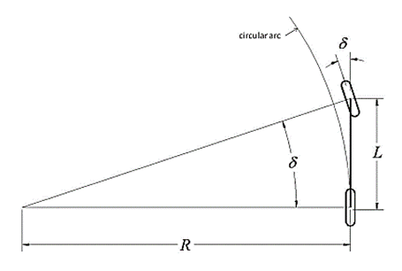
Figure 2: Bicycle Vehicle Model
tan(δ) = L/R …… (1)
where ‘δ’ is the steering angle of the front wheel, L is the distance between the front axle and rear axle (wheelbase) and R is the radius of the circle that the rear axle will travel along at the given steering angle.
The curvature of a circular arc from the rear axle position to a target point on the path ahead of the vehicle is calculated geometrically using the PURE PURSUIT technique. A look ahead distance is used to quantify inaccuracy ahead of the vehicle in this approach. The look-ahead distance ld from the present rear axle location to the intended path is used to establish the target point. In Figures 3a-b, the target point is depicted by a red dot. Only the target point location and the angle between the vehicle's heading vector and look-ahead vector may be used to estimate the vehicle's steering angle.

Figure 3a

Figure 3b
Applying the law of sines to Figure 4 results ld/(Sin(2α))=R/(Sin(π/2-α)) ld/(Sin(α)Cos(α))=R/(Cos(α)) ld/(Sin(α))= 2R K= 1/R=(Sin(α))/ld
where K is curvature of the circular arc. From equation (1) the steering angle can be written tan(δ) = L/R δ= 〖tan〗^(-1) KL δ(t)=〖tan〗^(-1) ((2LSin(α(t)))/ld)
A better understanding of this control law can be gained by defining a new variable, eℓd to be the lateral distance between the heading vector and the goal point resulting in the equation Put in equation (2), we get
Equation (4) shows that pure pursuit is a proportional steering angle controller with a gain of 2/ld2 that operates on a cross track error, a look-ahead distance in front of the vehicle, and a cross track error. In practise, the gain (look-ahead distance) is individually set to be stable at a number of constant speeds, resulting in the assignment of ld as a function of vehicle speed.
Tuning the Pure Pursuit Controller
The control rule may be revised to make tuning easier by scaling the look-ahead distance with the vehicle's longitudinal velocity. At four distinct constant velocities, namely 5 m/s, 10 m/s, 15 m/s, and 20 m/s, the pure chase controller is tested..
Results
**- Tracking of Lane Change Course **

Figure 4(a): Tracking for all Kdd values on Vx=5m/s

Figure 4(b): Tracking for all Kdd values on Vx=10m/s
On the Lane Change Course, 24 (For four Vx, six Kdd values) experiments are carried out. The impact of the tuning parameter on tracking performance is shown in Figure 5. The look-ahead distance grows as gain 'k' increases, and the tracking becomes less oscillatory. A shorter look-ahead distance allows for more precise tracking, whereas a larger distance allows for smoother tracking. A k value that is too little will create instability, whereas a k value that is too big will result in poor tracking. Another feature of Pure Pursuit is that if you maintain a sufficient look-ahead distance, you'll be able to "clip corners" when completing route turns. With Pure Pursuit, balancing the trade-off between stability and tracking performance is tough and will become course dependant. This is partly owing to the Pure Pursuit method's disregard for the path's curvature. Intuition would lead one to conclude that the path's curvature should affect both the look-ahead distance and the velocity (and perhaps even the current local cross track error).
- Cross Track Error Plots
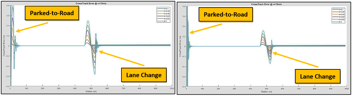
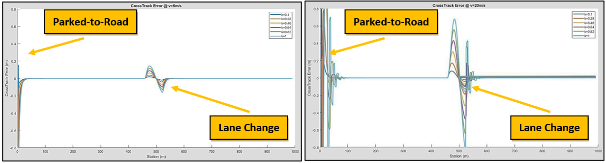
Figure 5 : (a) velocity at 5 m/s; (b) velocity at 10 m/s; (c) velocity at 15 m/s; (d) velocity at 20 m/s
Summary
Decreasing the look-ahead distance results in higher precision tracking and eventually oscillation, and increasing the look-ahead distance results in lower precision tracking and eventually stability.
The Stanley technique, as illustrated in figure 6, calculates cross track error from the centre of the front axle to the nearest route point (cx, cy) from the centre of the front axle (reference point). It considers both mistakes in direction and inaccuracies in position in relation to the path's nearest point. It employs a method for keeping the wheels aligned with the specified route, which involves setting the steering angle ‘δ’ equal to the heading inaccuracy, which is given as. θe = θ - θp where θ is the heading of the vehicle and θp is the heading of the path at (cx, cy). When cross track error is non-zero, the second term adjusts steering angle ‘δ’ such that the intended trajectory intersects the path tangent from (cx, cy) at kddVx(t) units from the front axle.

**Figure 6: Stanley Method Geometry **
An intuitive steering law is defined as under to: -
- Heading Control Law
- Correct heading error i.e steer to align heading with desired heading (proportional to heading error). δ(t) = ψ(t)
- Correct position error i.e. steer to eliminate cross track error. δ(t) = tan-1((ke(t))/(vf(t)))
- Obey maximum steering angle bounds. δ(t) ϵ [δ min, δmax]
- Combined Steering Law. Combining the above three equations results in steering control law, given as δ(t) = ψ(t) + tan-1((ke(t))/(vf(t))), δ(t) ϵ [δ min, δmax] where k is a gain parameter. It is clear that the desired effect is achieved with this control law: As cross track error increases, the wheels are steered further towards the path.
Case I.
- Large Heading Error
- Steer in opposite direction.
- The larger the heading error, the larger the steering correction.
- Fixed at limit beyond maximum steering angle.
- Assume no cross-track error.
Case II.
- Large Positive Cross Track Error tan-1((ke(t))/(vf(t))) ≈ π/2 π/2 ≈ ψ(t) + π/2
- As heading changes due to steering angle, the heading correction counter acts the cross-track correction and drive steering angle back to zero.
- The vehicle approaches the path, cross track error drops and steering angle command starts to correct heading error alignment.
- Error Dynamics. The error dynamics when not at maximum steering angle are ѐ(t) = -Vf Sin(ψ(t) – δ(t)) = -Vf Sin(tan-1((ke(t))/(vf(t)))) = (-ke(t))/√(1+〖((ke(t))/(vf(t)))〗^2 )
- For small cross track errors lead to exponential decay characteristics ѐ (t) = -k e(t)
Results
**- Tracking of Lane Change Course **

Figure 7: Tracking for all K values on Vx=5m/s - Cross Track Error Plots
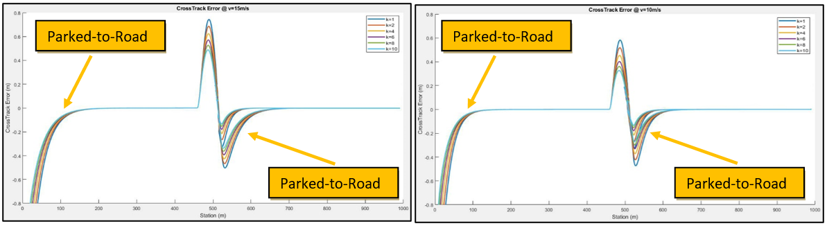
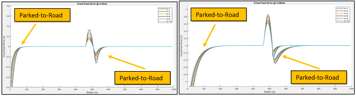
Figure 8 : (a) velocity at 5 m/s; (b) velocity at 10 m/s; (c) velocity at 15 m/s; (d) velocity at 20 m/s
CORRECTION: Right ones are "LANE CHANGE"
Problem Statement
Design a Controller (Lateral) and track Lane Change Course using designed Controller as per data / specifications of car given as under:- m = 1140.0 Kg b. lr = 1.165m c. lf = 1.165m cr = 155494.663 N /rad e. cf = 155494.663 N /rad f. Iz = 1436.24 kgm2
Controller Design
The plant used for controller design is linear and derived from the "bicycle" model state-space.
Results
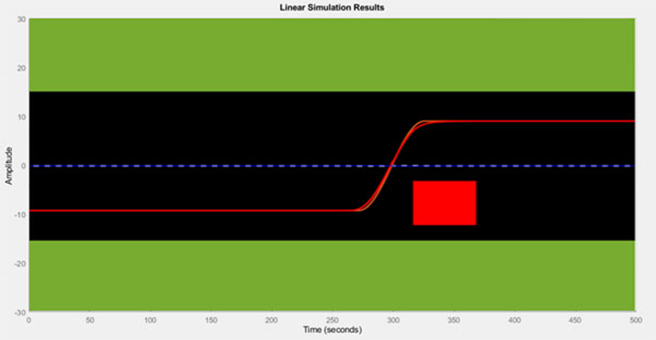
Summary
By inspecting the data, it's clear that raising the speed causes the zeros and poles on the complex plane to shift towards the imaginary axis. They're all type-2 systems, which means they're "structurally" unstable. This is clear since a system with zero steering angle as input would never get the lateral error (also known as lateral offset) to zero or maintain it constant.
We implemented three lateral control methods and same were examined for a project of trajectory tracking, with a hope to provide with some fundamental vehicle lateral control concepts. Thus, the theoretical learning focuses to enhance the knowledge however practical implementation of concepts and ideas lead to better understanding of the concepts and help build their confidence.


