
This repository contains the code of the monte-carlo simulation application presented by our Paper that we call RadField3D. This application aims to simulate a concentric x-ray beam, that can be rotated on a sphere with a certain radius around the center of the irradiated scene. RadField3D stores the radiation fields spatially resolved in an efficiently machine readable and interpretable file format that we refer to as RadFiled3D. The code of that file format is located here. Thanks to the Python API and pyTorch Integration, this application and RadFiled3D is suited to be used in machine learning. Therefore, RadFiled3D can be directly installed from PyPi using pip.
The validation dataset (measured and simulated) is available here:

You can build and install this application from source by using CMake and a C++ compiler. The CMake Project will be built automatically, but will take some time.
- C++20 Compiler
- g++ or clang for Linux
- MSVC or clang from Visual Studio 2022 for Windows
- CMake >= 3.24
- Python >= 3.10
- Geant4 >= 11.0 (validated on 11.0.0), including its data packages (see Running)
- Optional:
- OpenGL (only needed for the
WITH_GEANT4_UIVISvisualiser build)
- OpenGL (only needed for the
Just execute CMake on the CMakeLists.txt from the root of the project and set the following CMake options:
- WITH_GEANT4_UIVIS (
ON/OFF, defaultOFF): Build with the Geant4 OpenGL UI/visualiser. If enabled, RadField3D runs single-threaded and shows a window where the path of each particle can be viewed; otherwise no window is shown and all available cores are used. - BUILD_TESTS (
ON/OFF, defaultOFF): Build the Google Test suite.
CMake locates Geant4 via find_package(Geant4); if it is not on the default search path, point CMake at your
install with -DGeant4_DIR=<geant4>/lib/cmake/Geant4 (and -DCLHEP_DIR=<clhep>/lib/CLHEP-<ver> if CLHEP is
external). Only the OBJ and STL assimp importers are built (the only geometry formats used).
All other dependencies are fetched and built automatically on the first configure (network access required): Eigen,
Assimp, nlohmann/json, GoogleTest (tests only) and, for voxelizing the geometry, OpenVDB
(core library only, CPU-only, Apache-2.0) with oneTBB (Apache-2.0). An
already installed oneTBB (TBBConfig.cmake) or OpenVDB (FindOpenVDB.cmake on CMAKE_MODULE_PATH) is used instead
of fetching it. Both are linked statically, so the built binary needs no extra runtime libraries.
cmake -S . -B build            # add -DGeant4_DIR=... if Geant4 is not auto-found
cmake --build build -j # produces bin/RadField3DEvery run seeds Geant4's random engine from the system time (mixed with the process id), so runs are independent of each other; all random numbers of a run, including the sampled primary energies and directions, come from that engine. The seed is printed and stored in the field metadata as random_seed, and --append refuses a run whose seed equals the file's.
RadField3D needs the Geant4 data packages at runtime. Install them with your Geant4 build and make the
G4*DATA environment variables available before running — e.g. source <geant4-install>/bin/geant4.sh, or set
them from geant4-config --datasets. If a required dataset is missing, RadField3D prints exactly which
G4*DATA variable is unset and exits, instead of crashing inside Geant4. ./RadField3D --help works without
any datasets.
Datasets can be generated by calling RadField3D multiple times or using the DatasetGenerator written in Python. The spectra loading from the python DataGenerator requires pyTorch. Every 1 million primary particles, RadField3D will store a intermediate result to the disk to make sure that no progress is lost in case of possible errors.
The commandline interface of RadField3D can be printed by calling: ./RadField3D --help or .\RadField3D.exe --help.
The parameters are the following:
- out: The output path of the apllication. Must end with
.rf3otherwise the extension will be added. - max-energy: Maximum energy to consider for the energy spectrum in each voxel. Value must be given in eV.
- source-phi: The rotation in degree inside the horizontal plane (about Y), see Source angles.
- source-theta: The tilt in degree about X that follows it, see Source angles.
- source-psi: The turn in degree of the C-arm structure (meshes of Type
CArm) about the beam axis. The beam and its field do not change. Default: 0. - source-distance: Radius of the roation sphere in meter (Equals the distance of the source from the center of the scene).
- world-dim: Dimensions of the World in meter provided as a string looking like this: "x y z". The used source can be located outside this tracking volume.
- particles: Maximum count of particles (photons) to track.
- voxel-dim: Dimensions of each voxel along each dimension in meter. Voxels are supposed to be cubes, hence this parameter only accepts one float value.
- energy-resolution: The used energy resolution in eV that should be used as the bin width when scoring photon energy spectra.
- source-shape: The used source shape to sample rays from. Can be one of:
cone,rectangleorellipsoid. - source-opening-angle: The opening angle to use for the ray sampling from the source.
- For
cone: One single value for the half opening angle in degrees. - For
ellipsoid: Two values for the half opening angle in degrees along x and y, each in (0, 90). Rays are uniform per solid angle inside the elliptical cone. - For
rectangle: Two values for the rectangle extents in meter insource-distancemeter away from the source (so in the center of the scene). The source is a point source behind a rectangular collimator: rays are uniform per solid angle, so the photons per area of that plane fall off towards the edges as cos³θ.
- For
- tracing-algorithm: The used algorithm to find intersected voxels for a given particle path. Can be one of
sampling,bresenhamorlinetracing(default).linetracingcounts every voxel a step touches;samplingmisses voxels that an oblique step only clips, which lowers the flux of oblique photons (about 7 % in a 20 × 20 cm² beam at 64 cm). - geom: The path to the geometry file. The geoemetry can be provided by all file formats supported by Assimp like
.obj,.fbxor.stl. For each geometry file, one can specify a world scene description file named with the pattern:[base-file-name].descon the same folder as the geoemtry file. - world-material: Material of the world. Default: Air.
- spectrum: The path to a x-ray spectrum in .csv-format. The CSV-file should have the form column 1: the centre energy of a bin and column 2: relative photon counts for this bin (see Spectrum files). The input distribution will be normalized to a integral of one.
- autosave-interval: Store the field every N particles while the simulation runs (default 1e7, 0 disables auto-saves). Raise it for long runs with large layers (e.g. a fine angular resolution), where every save writes the whole file.
- append: If a file with the specified name and matching simulation setup is already present, this run is combined with it as if both had been one run: flux and angular flux are averaged weighted by the primary particles of each, the spectra are mixed per voxel weighted by each run's flux, the statistical errors are combined accordingly, and the primary particle counts and the
tube_spectrumcounts add up. The file's geometry channel is kept. All arithmetic runs in double precision; a result that does not fit the stored float32 type, an unknown layer or a different setup abort the append and leave the file unchanged. During an--appendrun, auto-saves go to a checkpoint<out>.partial-<token>next to the output file instead of the output itself, which receives the run exactly once when it finishes; the checkpoint is then removed. If a run crashes, its checkpoint is a complete field of the particles simulated so far. If the final append fails, the whole run is written to the checkpoint and the program exits with an error. - geom-desc: Path to the geometry world-description JSON (see below). Default: the geometry file with its extension replaced by
.desc. - cpu-count: Number of CPU cores (worker threads) to use. Default:
-1(all available cores). - angular-resolution: Optionally enables an extra per-voxel layer that captures the angular distribution of the flux. Provide as
"phi theta"segment counts. - path-length-weighting:
on(default) oroff. With the line tracer, flux, spectrum, angular bins and vMF lobes hold the incident radiation weighted by the path length inside each voxel (track-length estimate): a corner clip counts almost nothing, an axis-parallel crossing 1, and no direction is favoured by how many voxels it grazes. The voxel a step starts in is left out (after an interaction the radiation there leaves the voxel). The flux unit is thenvoxel edges / primary_particles(path length in voxel edges per primary); isotropic scatter comes out about a third lower than withoff, which counts every touched voxel once (the behaviour before 1.2.0).--appendrefuses to mix the two. - directional-lobes: Optionally learns, per voxel of the
scatter_fieldchannel, the directions of travel as a mixture of at most N von Mises–Fisher lobes (1–8) and stores it as layervmf_lobes(per lobe: weight as share of the voxel flux, mean direction, concentration κ). Lobes that describe the same source are merged, so a voxel lit by one source keeps a single lobe. Unlike direction bins it gives the radiance in an exact direction with 5·N values per voxel.direct_beamgets no lobes, its direction is the line from the focal spot. Needs a RadFiled3D version with the vMF layer type;--appendrefuses files with this layer. - statistical-error-threshold: Relative statistical error at which the simulation stops early. Default:
0.1(10%). Compared with the 95 % quantile (see statistical-error-enforcement-ratio) of the per-voxel relative standard error of the scatter flux, computed history by history (stored as layererror). - statistical-error-enforcement-ratio: Fraction of voxels that must be below the error threshold before the run stops early. Default:
0.95(95%). - gui: Show the Geant4 GUI. Only available in a
WITH_GEANT4_UIVISbuild; ignored otherwise.
Run ./RadField3D --help for this list at any time (it works without the Geant4 datasets).

The patient lies along Z (head at +Z), Y points up and X runs across the table. The beam direction is
d = Rx(θ)·Ry(φ)·(0, 0, −1) = (−sin φ, cos φ·sin θ, −cos φ·cos θ), and the source sits at −d · source-distance.
φ = 0°, θ = 90° is the base pose: tube under the table, beam pointing up along +Y.
The collimated field is oriented like on a C-arm: the source frame is a turn of the arm about the patient's long axis Z after a tilt about X, so the field never rolls about the beam. Its x side (the first value of a rectangle's size) is always horizontal, x = d × Z, and its y side lies in the plane of d and Z; in the base pose x runs along X and y along Z. With the beam along ±Z the turn about Z is taken as zero. Fields written before this frame carry no xray_tube_source_frame metadata; their field was the shortest rotation from −Z onto d and rolled about the beam with φ.
ψ turns only the C-arm's own structure about the beam, right-handed about d. It is the extra degree of freedom of a real C-arm (e.g. the C swung from the head end to the side): the primary beam, the collimator, the image detector and the tube housing stay where φ and θ put them, but the arm's mass moves and with it the scatter it adds to the field. It is stored as c_arm_psi_deg, so a model trained on these fields needs it as an input next to φ and θ.
The DatasetGenerator samples beam directions uniformly on the sphere: within a source_angle_phi range, φ takes the density |cos φ| (the area element of this parametrisation is |cos φ| dφ dθ), and θ stays uniform in its range. Uniform φ would crowd the beams at the poles of the parametrisation, ±X: lateral beams about 2× denser than uniform, beams in the YZ plane about 0.65×. Datasets generated before 2026-11-11 were sampled that way.
./RadField3D --out test.rf3 --max-energy 1.5e+4 --source-phi 0 --source-theta 0 --source-distance 2 --world-dim "1 1 1" --particles 1e+7 --voxel-dim 0.02 --geom <a-geom-file> --spectrum <spectrum.csv>
The geometry description file contains the information how the meshes of the geometry file are nested inside eachother and which material each mesh volume has. Additionally, a transformation for each mesh can be supplied. The file shoud have the JSON-Format. Example:
{
    "mesh_name": {
        "MaterialName": "G4_TISSUE_SOFT_ICRU",
        "Type": "Patient", // free text; "Patient" may be used by one mesh only
        "Transform": {
            "Rotation": {
                "X": 0,
                "Y": 3.14159265359,
                "Z": 0.0
            },
            "Translation": {
                "X": 0.0,
                "Y": 0.0,
                "Z": 0.0
            },
            "Scale": {
                "X": 1.0,
                "Y": 1.0,
                "Z": 1.0
            }
        }
        "Children": {
            "child_name_name": {
                "Type": "Organ",
                "MaterialName": "G4_LUNG_ICRP",
                "Transform": {
                    "Rotation": {
                        "X": 0,
                        "Y": 0.0,
                        "Z": 0.0
                    },
                    "Translation": {
                        "X": 0.0,
                        "Y": 0.0,
                        "Z": 0.0
                    },
                    "Scale": {
                        "X": 1,
                        "Y": 1,
                        "Z": 1
                    }
                }
            },
        }
    }
}
With mesh_name and child_name_name name being the name of the mesh as exported by the geometry file. MaterialName can be one of the Geant4 Materials, but it is more error prune as Water will be corrected to G4_WATER, if the prior was not a valid material.
Type is a freely assignable category of the mesh, e.g. "Patient", "Shield" or "Table". Types are matched case-insensitively and stored in lower case ("Shield" and "SHIELD" are the same type shield) and may have at most 63 characters. A mesh without a Type takes the type of its parent (recursively), a root mesh without one is of type unknown; a child with its own Type is a separate type. At most one mesh may declare the type patient; its translation is what the DatasetGenerator records as the patient translation. Descriptions using the former boolean "Patient": true are still read as "Type": "Patient" ("Patient": false declares no type).
Three types are reserved for meshes on the C-arm and are turned with the beam for every field. Model them in the base pose: tube under the table, beam pointing up along +Y, which is phi = 0°, theta = 90°.
-
"ImageDetector"is modelled relative to the isocentre, e.g. a detector plate above the table. It keeps its distance to the isocentre, stays opposite the tube and faces the beam. With"IsocenterDistance": { "Min": 0.45, "Max": 0.62 }its distance follows the collimation instead: its entrance face moves as far out as the beam still fits on it, within these limits (metres). Small fields leave the plate partly unlit atMax; keep the collimation small enough that the beam fits atMin. -
"XRayTube"is modelled around the focal spot placed at the origin, e.g. a tube housing or collimator. It moves with the focal spot. -
"CArm"is the arm itself (the C, its rail and covers), modelled relative to the isocentre like the image detector, e.g. with its back towards the head end. It turns with φ and θ about the isocentre and in addition by ψ about the beam axis; it is never fitted to the beam. Draw it in the base pose with the isocentre at the origin: the C lies in the YZ plane around the patient's head end (+Z), its ends under the tube (−Y) and behind the image detector (+Y), and nothing of it in the primary beam. Give it a material that stands in for its structure, e.g.CArm_AlPolymer.python tools/add_carm_mesh.py <geometry.obj>appends such an arm to a geometry and its.desc(defaults: Siemens Artis Q with 78.5 cm focus–isocentre distance, C-arm depth 94 cm).A real C-arm cannot take a pose in which it runs into the table, the patient or the room, and Geant4 cannot transport through overlapping volumes. RadField3D therefore checks the placed arm against all other volumes before simulating; if they overlap it writes no field and exits with code 3, and the DatasetGenerator drops that sample. The analytical simulator does not check this.
The former Source/SourceOffsets keys are no longer supported.
Before the simulation starts, RadField3D voxelizes the placed geometry onto the grid of the radiation field and stores it as the channel geometry of the .rf3 file. Every mesh type gets its own 8-bit layer named like the (lower-case) type, e.g. patient, holding 255 where a voxel overlaps any mesh of that type and 0 elsewhere; all meshes of one type share their layer. A voxel counts as overlapping when a part of it with non-zero volume lies inside the mesh, so meshes thinner than a voxel (e.g. shields) are still marked. Meshes must be closed up to gaps smaller than a voxel.
The geometry is written once when the file is created; later saves (auto-saves or --append runs) only update the radiation channels and the metadata and keep the stored geometry.
After installing the needed pyTorch (CPU or CUDA version doesn't matter) and other required modules (from requirements.txt), one can call the DatasetGenerator from ./tools/create_dataset.py. The fields it creates carry the voxelized geometry written by RadField3D (see Voxelized geometry).
The arguments of the generator are working similar like the direct RadField3D parameters, but slightly extended.
Parameters:
- dest: Distination path to a folder, where the fields will be stored to.
- fields: Number of fields to calculate.
- Emin: Only use when no Spectra are defined. Specifies the lower end of the source energy sampling in eV.
- Emax: Specifies the upper end of the source energy sampling in eV. Which will be used for the upper bound of the voxel spectra stored.
- particles: Maximum count of particles (photons) to track.
- geometry: The path to the geometry file. The geoemetry can be provided by all file formats supported by Assimp like
.obj,.fbxor.stl. For each geometry file, one can specify a world scene description file named with the pattern:[base-file-name].descon the same folder as the geoemtry file. See the previous example of the world description file. - voxel_size: Dimensions of each voxel along each dimension in meter. Voxels are supposed to be cubes, hence this parameter only accepts one float value.
- world_size: Dimensions of the World in meter provided as a string looking like this: "x y z". The used source can be located outside this tracking volume.
- binary: Path to the RadField3D binary to execute.
- spectra: path to a single spectra file or folder containing multiple spectra to sample one spectrum from. Single spectrum files can be .csv-files like described prior or .spectrum-files that will be loaded as torch tensors. Used spectrum files will be copied in to the destination file and linked with the radiation field files.
- source_distance: Radius of the roation sphere in meter (Equals the distance of the source from the center of the scene).
- source_shape: The used source shape to sample rays from. Can be one of:
cone,rectangleorellipsoid. - source_angles: The angles from which the source is facing the center (phi and theta angle in degree).
- source_opening_angle: The opening angle to use for the ray sampling from the source.
- For
cone: One single value for the half opening angle in degrees. - For
ellipsoid: Two values for the half opening angle in degrees along x and y, each in (0, 90). Rays are uniform per solid angle inside the elliptical cone. - For
rectangle: Two values for the rectangle extents in meter insource-distancemeter away from the source (so in the center of the scene). The source is a point source behind a rectangular collimator: rays are uniform per solid angle, so the photons per area of that plane fall off towards the edges as cos³θ.
- For
- clean: Issues to first remove all radiation field files that already exist and do not append to them.
- bin_count: Sets the energy resolution according to the desired bin count and maximum energy.
- tracer_algorithm: The used algorithm to find intersected voxels for a given particle path. Can be one of
sampling,bresenhamorlinetracing(default). - autosave_interval: Passed to the binary as
--autosave-interval(default 1e7 photons, 0 turns auto-saves off). Every save writes the whole file and pauses the scoring, so a small interval slows long runs (1e8 photons with saves every 1e6 took ~20 instead of ~12 minutes). - statistical_error_threshold: Stops a field early once the binary's estimate of the relative statistical error falls below this value.
0(default) turns the early stop off, so every field gets exactlyparticlesphotons; the binary on its own stops at0.1unless told otherwise. A"StatisticalErrorThreshold"metaparameter sets it for a whole dataset. - join_channels: Optional post-simulation step. Joins the
direct_beamandscatter_fieldchannels into a single per-primary field (removing the two originals) to roughly halve the per-field storage. The flux is summed (staying per primary particle); the spectrum is combined as a flux-weighted per-voxel mix and renormalized per voxel; the statistical error is the mean; any other channel (e.g. the voxelized geometry) is kept unchanged. - sequence_file: Optional: Allows to load some of the options sequentially from a JSON-File to automate specific dataset configurations under specified conditions.
- dataset_definition: Provide the path to a JSON file containing a whole dataset generation definition. This overrdides all other parameters except for
--dest,--binaryand--cluster_node_partition. An Example can be found below. - cluster: An optional cluster submenu for specialized cluster actions
- node_partition: Optional. Only used when
sequence_fileis set. Allows to determine which section of a sequence file should be processed by this process. Useful when multiple instances are run on a cluster. Specify in the form of: "m" "n" where n is the current node ID ([0..(m-1)]) and m is the total node count. - generate_batch: Generate cluster batch files
- type: Type of the cluster system ('slurm')
- node_initialization_batch_path: Path to a batch file that should be executed on the cluster nodes before the calculation starts
- node_partition: Optional. Only used when
python tools/create_dataset.py --dest <path-to-dataset-folder> --binary <path-to-RadField3D-executable> --dataset_definition <path-to.json> cluster --node_partition <m> <n>
{
    "Metaparameters": {
        "MaxEnergy": 1.5e+4,
        "GeometryFile": "<path-to-a-geometry-file.obj>",
        "Particles": 200000,
        "TracerAlgorithm": "linetracing",
        "BinCount": 32,
        "WorldDim": [1, 1, 1],
        "VoxelSize": 0.02,
        "nSamples": 500,
        "WorldMaterial": "Air"
    },
    "Parameters": [
        {
            "name": "source_distance",
            "values": [2.5, 2.0, 1.5]   // This is a list to sample randomly from
        },
        {
            "name": "source_angle_phi",
            "range": [-90, 90]          // This is a range to sample uniform within
        },
        {
            "name": "source_angle_theta",
            "value": 0                  // This is a fixed value that never changes
        },
        {
            "name": "source_angle_psi",
            "range": [-90.0, 90.0]      // Turn of the C-arm mesh about the beam; 0 when left out
        },
        {
            "name": "source_opening_angle",
            "value": 5
        },
        {
            "name": "source_shape",
            "value": "cone"
        },
        {
            "name": "source_spectra",
            "value": "<path-to-a-spectra-file-or-folder>.spectra/.csv"
        }
    ]
}
Every entry in Parameters is sampled once per field and accepts one of: "value": x (fixed), "values": [a, b, c] (a discrete set sampled uniformly) or "range": [min, max] (a continuous range sampled uniformly).
For a rectangle source, source_opening_angle is the pair of beam extents in metres at source_distance — i.e. the collimated field size in the centre of the scene — and additionally supports a range so the collimation can be sampled continuously. A range is given as a min vector and a max vector [[x_min, y_min], [x_max, y_max]]; each axis is sampled independently between the two corners (so non-square collimation is allowed):
"value": "0.10 0.10"(or"value": [0.10, 0.10]) — a fixed 10 cm × 10 cm field."range": [[0.05, 0.05], [0.20, 0.20]]— sample x and y independently within 5–20 cm."range": [[0.05, 0.10], [0.20, 0.15]]— an asymmetric range: x within 5–20 cm, y within 10–15 cm.
Patient/object motion is sampled per field via a top-level GeometryTransformations block. A group moves several meshes rigidly by one sampled offset, e.g. patient and table: { "patient_on_table": { "Meshes": ["patient", "HardDesk"], "Translation": { "X": [-0.2, 0.2], "Y": [-0.285, -0.04], "Z": [-0.7, 0.7] } } }; an entry named after a single mesh sets per-axis Translation/Rotation/Scale ranges for that mesh, e.g. { "patient": { "Translation": { "Z": [-0.5, 0.5] } } }. See example/dataset_ds_04.json with example/DS04-Angio.obj/.desc.
An optional post-simulation step is configured from Metaparameters: "JoinChannels": true merges the direct_beam and scatter_field channels into one per-primary field to roughly halve the stored size (see the join_channels generator option above). The stored field size is set directly by WorldDim / VoxelSize (e.g. WorldDim [1.28, 1.28, 1.28] at VoxelSize 0.02 gives 64³); the geometry may be larger than the world.
{
    "Metaparameters": {
        "MaxEnergy": 1.5e+4,
        "GeometryFile": "<path-to-a-geometry-file.obj>",
        "Particles": 200000,
        "TracerAlgorithm": "linetracing",
        "BinCount": 32,
        "WorldDim": [1, 1, 1],
        "VoxelSize": 0.02
    },
    "ParameterSets": [
        [
            {
                "name": "source_distance",
                "value": 2.5
            },
            {
                "name": "source_angle_phi",
                "value": 0
            },
        ],
        [
            {
                "name": "source_distance",
                "value": 2.0
            },
            {
                "name": "source_angle_phi",
                "value": 0
            },
        ],
        [
            {
                "name": "source_distance",
                "value": 1.5
            },
            {
                "name": "source_angle_phi",
                "value": 0
            },
        ]
    ]
}X-ray spectra for the radiation source can be passed to the simulation by spectra files. When using the python dataset generator those can be of two types determined by their file extension:
- *.spectrum files will be interpreted and parsed as pickle files of pyTorch tensors. Those are converted to CSV files, readable by the RadField3D application itself. The first column shall be the centre energies of the bins in eV (SpekPy's mid-bin energies) and the second column the probability of a photon of that bin. Each *.spectrum file should be accompanied by a *.info file replacing the .spectrum extension that holds a JSON document that defines the origin configuration that created this spectrum. RadField3D only requires that document to contain a "energy" field in eV that defines the maximum tube energy.
- *.csv will be interpreted and used as ASCII CSV files. Here the first column is containing the centre energies of the bins and the second column the probability of a photon of that bin. It is required, that the column has a unit of eV, keV or MeV declared to ensure correct handling of the spectrum.
For a direct call of RadField3D, only ASCII *.csv files can be used.
In any case, RadField3D will normalize the spectrum to ensure it to be a probability distribution. Each listed energy is the centre of a bin that reaches halfway to the neighbouring energies (the first and last bins reach as far outwards as inwards), and energies are sampled uniformly within their bin. This matches SpekPy's output and the tube spectrum RadField3D stores in every field, so a spectrum extracted from a field reproduces the original one.
Energy[MeV]    Fluence[]
0.01500E+00, 6.70777566040744E-12
0.01600E+00, 3.94509821006659E-10
0.01700E+00, 1.08557495078525E-08
0.01800E+00, 1.577541987836E-07
Please note, that colons (,) will be converted to spaces and it is just required to seperate the columns by using spaces.
Please note, that the dataset generator tool only requires the energy field to be set to the maximum energy of the tube in eV.
{
    "energy": 100000.0,
    "anode_angle_deg": 35,
    "target_material": "W",
    "layers": [
        {
            "material": "Be",
            "thickness_mm": 1
        },
        {
            "material": "Cu",
            "thickness_mm": 4.028
        },
        {
            "material": "Al",
            "thickness_mm": 0.151
        }
    ]
}You can specify any material included into Geant4 from the NIST Materials Database.
Additionally, MaterialSolver::init_custom_materials() from G4SceneConstructor.cpp exports the following additional Materials.
| Name | Composition |
|---|---|
| Polyamide | 57% H, 31% C, 5% N, 5% O ; ρ = 1.14 g/cm^3 |
| CarbonFiber | 60% C, 40% Epoxy ; ρ = 1.6 g/cm^3 |
| ThoraticSpongiosa | Approximating ICRU Report 46 for the Thoratic spine ; ρ = 1.074 g/cm^3 |
| CsI (Cesium Iodide) | 50% Cs, 50% I (source); ρ = 4.51 g/cm^3 |
| PU_foam (Polyurethan foam) | 48% C, 36% H, 10% O, 6% N ; ρ = 0.05 g/cm^3 |
| CArm_AlPolymer | 78% G4_Al, 22% G4_POLYCARBONATE (by mass) ; ρ = 0.51 g/cm^3: a hollow aluminium box section (~10 × 20 cm, 5 mm walls) under ~3 mm polycarbonate covers, smeared over a solid C-arm mesh |
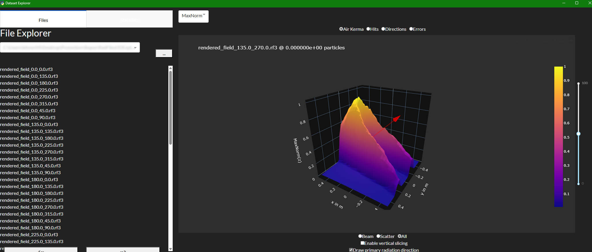
For viewing the results of the simulation and analyzing whole datasets, we provide the so called RadFiled3DExplorer. That little python program offers a GUI to view radiation fields generated with our simulation software. You find the project here.
@article{Lehner_2025,
    doi = {10.1088/1361-6498/add53d},
    url = {https://dx.doi.org/10.1088/1361-6498/add53d},
    year = {2025},
    month = {may},
    publisher = {IOP Publishing},
    volume = {45},
    number = {2},
    pages = {021508},
    author = {Lehner, Felix and Lombardo, Pasquale and Castillo, Susana and Hupe, Oliver and Magnor, Marcus},
    title = {RadField3D: a data generator and data format for deep learning in radiation-protection dosimetry for medical applications},
    journal = {Journal of Radiological Protection}
}